
In attempting to explain ML models, there are two general approaches: explanation that targets the global model behavior or the local behavior (i.e. explain the decision of the model around an instance). One example of global explanation is the feature importance method that comes with many tree-based estimators. However, the feature importance value is derived from impurity-based metric (measure of homogeneity of the labels in the node), and it is biased against low cardinality features(feature with small number of unique values). It can also assign misleading importance to features that don't predict well on new test data due to overfitting of the model[1]. On the other hand, permutation feature importance examines how the permutation of a feature decreases the model performance, but it doesn't capture how much of the output variance is explained by that feature. There's also debate on whether to apply permutation feature importance on the training dataset or the test dataset[2].
Enter localized model explanation, such as LIME and SHAP values.
The premise of SHAP is to calculate the average marginal contributions of features across all possible permuted subsets. I've written an old blog on LIME before, and one of the drawbacks is that LIME doesn't work for regression model. With SHAP values, it works beautifully for both classifier and regression models. KernelSHAP approximates the SHAP values via marginal expectation, and is very similar to LIME except for the weighting mechanism. On the other hand, TreeSHAP computes the actual SHAP values based on conditional expectations.
TreeSHAP - order matters
TreeSHAP is used to explain a single prediction instance in terms of marginal contributions from sets of permuted input features in the decision tree model. It's marginal because it's the contribution to some reference baseline value, and the governing equation for the SHAP value of feature i is as follows [3]:
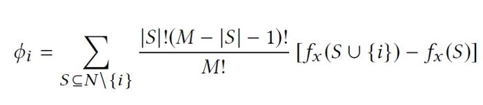
= the size of total number of features
= a subset of features that excludes the i-th feature used in one iteration
= the size of a given subset
and are
the conditional expectations for feature vector with the i-th
feature and without, respectively
(for TreeSHAP,
To illustrate how TreeSHAP works, I will use an example from a work project I did. A Gradient Boosted model was used to predict malnutrition rate based on explanatory variables like precipitation(CHIRPS), population, Consumer Price Index (CPI), consumption expenditure, etc. There's total of 6 variables, so that would be 720 permute sequences. For simplicity, I will only show the example with 3 variables: precipitation, CPI, and population, on one gradient boosted tree.
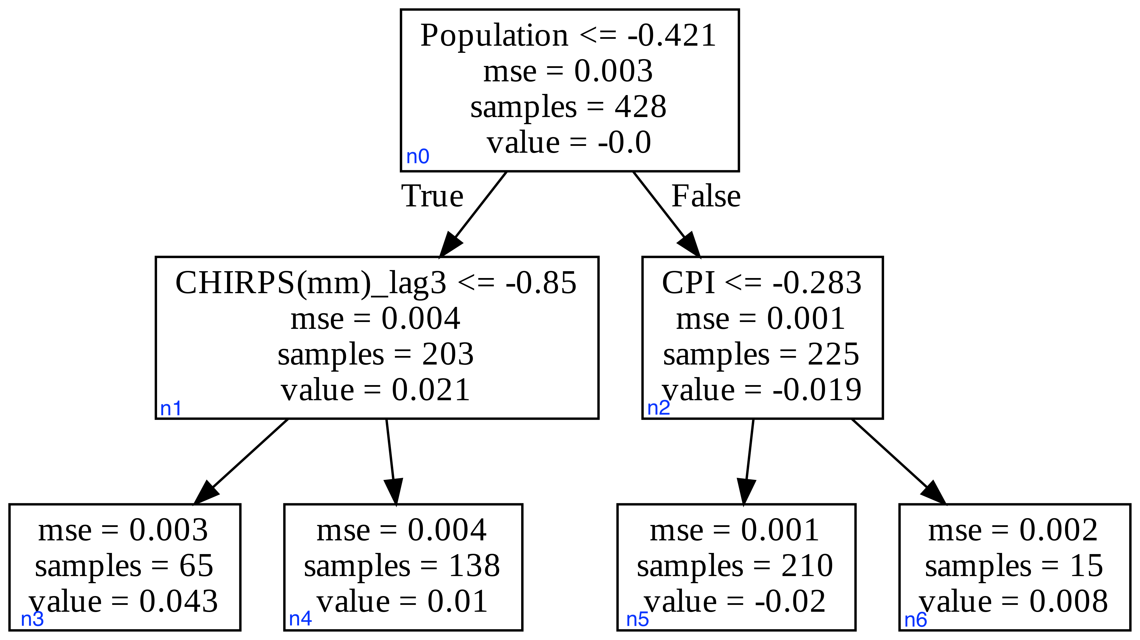
To start, we first need to compute the SHAP value for the null model, and that's the weighted average of the leaf node values (output). The given instance is Population= -0.20 CPI= -0.35 CHIRPS = -0.10. From the tree in Fig.1., the average would be (0.043*65+0.01*138+(-0.02)*210+0.008*15)/(65+138+210+15) = 0.00022
Next, we extract the prediction conditioned on a subset of the feature vector, and calculate the marginal contribution as each feature is added in order. It's worth noting that the result we get will depend on the order of the sequence. For the first example, we will start with the subset that is Population -- CHIRPS -- CPI, where we add the feature Population to the null model. The value of -0.20 for Population leads to the right child node (n2), where the feature CPI is used to split. Since CPI is not added as a feature at this stage, we simply take the weighted average of the child nodes from this point, which is (-0.02*210+0.008*15)/(225)=-0.018, so θpop_1 = -0.018-0.00022 = -0.0182. Then we add the feature CHIRPS to it, however for this test instance it doesn't use CHIRPS to split it, the predicted value is the same as before adding CHIRPS, so θchirps_1 = 0. Continuing with the sequence, we add the feature CPI and that led to the prediction of -0.02, so θCPI_1 = -0.02-(-0.018) = -0.002.
Let's look at what happens when we try a new permutation of CHIRPS -- Population -- CPI. In this case scenario, CHIRPS didn't show up in node n0, so we take the average of the child nodes n1 and n2, (prediction_n1*203+prediction_n2*225)/(203+225). For prediction_n1, the CHIRPS value is used to arrive at the prediction of 0.01. For prediction_n2, it's the same as before, (-0.02*210+0.008*15)/(225)=-0.018. Therefore, prediction with CHIRPS as the only feature is (0.01*203+(-0.018)*225)/(203+225)=-0.0047, so θchirps_2=- 0.0047- 0.00022=-0.00492. Next, adding population results in prediction_n2 of -0.018, θpop_2=-0.018-(-0.0047)= -0.0133. Finally, adding CPI gives a prediction of -0.02, so θCPI_2=-0.02-(-0.018)=-0.002.
The process is repeated for all the permute sequences of all the subsets () in order to estimate the average θi, where i is a given feature; the summation of the θis equals to the final prediction value. This example only shows one tree, but for the whole ensemble tree model, each prediction value would be derived by running through all the tree estimators. The SHAP package developed by Lundberg et al runs in time and memory (an improvement over conventional method that ran in exponential time), where is the number of trees, is the max number of leaves in any tree, is the maximum depth of any tree, and is the number of features[3].
In Python, we can leverage the SHAP package to easily run TreeSHAP on a trained model. Fig.2(a) shows the few lines of code to generate the SHAP plot, where it displays the top features with the highest contributions for one test sample. The summary plot in Fig.2(b) shows a more "global" snapshot of the distriubtion of impact. In this case, higher population (red dots) tends to correlate with lower value of malnutrition rate.
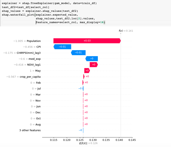
(a)
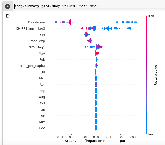
(b)
Convolutional Neural Net (CNN) transparency with Grad-CAM
CNN is the building block of many AI models out there. While it's proven to be versatile and powerful, it's often difficult to understand how all the internal workings of the model yields the output, especially when you consider the breaking of linearity within the convolutional feature maps through nonlinear functions (e.g. ReLU).
It is well documented that CNN model often overfit during training. This means it's "memorizing" features on the training set data that are not really
the relevant features, so the model doesn't perform well on new test data. One way to validate a CNN model is by visualizing the activation features
through saliency map (offered by keras-vis),
which identifies the pixels/area that the model attends to when predicting the target.
The saliency map hightlights the parts of the image that are most impactful in model prediction; it maps the relationship of the input to the generated
prediction by computing the gradient of the output with respect
to the input pixel array when the input is perturbed [4].
Despite its usefulness, saliency map is not class discriminative[5]. It means the same spots can be highlighted that correlates with various class labels, so those features are not specific to the prediction of any one class. Grad-CAM was created to solve this problem, because it aims to highlight only the regions that correspond to the label of interest. Fig.3. shows the clever way for generating the Grad-CAM heatmap.
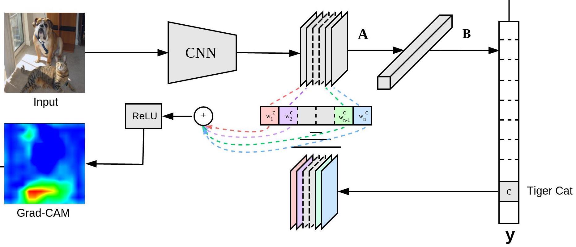
The guiding principle is that it backpropagates the gradient of the class prediction with respect to a pre-determined activation layer, followed by global average pooling to estimate the relative importance of each feature map. Based on the importance value, a weighted combination of those feature maps are created as a heatmap. Within this heatmap, the positive values correspond to pixels that contributes to the prediction of the class of interest. In the last step, the heatmap passes through the ReLU function to drown out negative values which correspond to pixels that contributes to the prediction of other classes (not the class of interest).
Inspired by the examples from the Keras blog and jacobgil, I tred out Grad-Cam on an image of a jelly fish with the following function to calculate Grad-CAM.
This function can be used on any DL model classifier that has convolution and activation layers. The input layer_name is the
name of the activation layer (the ReLU) post convolution. For this example, I ran Grad-CAM through the last 8 activation layers in pretrained Xception model and compiled the heatmaps into a
video clip (see below). As displayed in the animation, during the earlier convolutions the model is looking at the environment around the jelly fish, as it progresses it has "learned" to look at the right spots at the final
activation layer (Activation map
8).
The concept of Humble AI
Companies like GE and DataRobot have advocated for tools branded as Humble AI, which helps the user to assess the risk and reliability of a model and implement custom rules as guardrails. Having tools like SHAP values and Grad-CAM are useful in evaluating the trust worthiness and potential biases of the model. A user can take advantage of the SHAP output, and check for outliers in the top contributing features before making an inference, or visually inspect a gradient heatmap to make sure the model is looking at the right spot for making a label prediction.
Most of the recent improvements are targeted at machine learning models and convolutional models, but there's also progress made for NLP models such as exBERT for probing transformer representations. With the recent criticisms of harmful biases rolled out by GPT-3, it presents an urgent need for explainable AI tailored to NLP models. Given the far-reaching power of AI, model explainability would soon be a requisite for commercial applications and deployment.
REFERENCES
[1]Scikit-learn documetation, Relation to impurity-based importance in trees ,https://scikit-learn.org/stable/modules/permutation_importance.html#permutation-importance
[2]Molnar, C. Interpretable Machine Learning, https://christophm.github.io/interpretable-ml-book/feature-importance.html
[3]SM Lundberg, GG Erion, SI Lee, Consistent individualized feature attribution for tree ensembles, arXiv preprint arXiv:1802.03888
[4]Visualizing Keras CNN attention: Grad-CAM Class Activation Maps, 2019, https://www.machinecurve.com/index.php/2019/11/28/visualizing-keras-cnn-attention-grad-cam-class-activation-maps/
[5]Selvaraju, R. R., Cogswell, M., Das, A., Vedantam, R., Parikh, D., & Batra, D. Grad-CAM: Visual Explanations from Deep Networks via Gradient-Based Localization. 2017 IEEE International Conference on Computer Vision (ICCV). doi:10.1109/iccv.2017.74