Data preprocessing
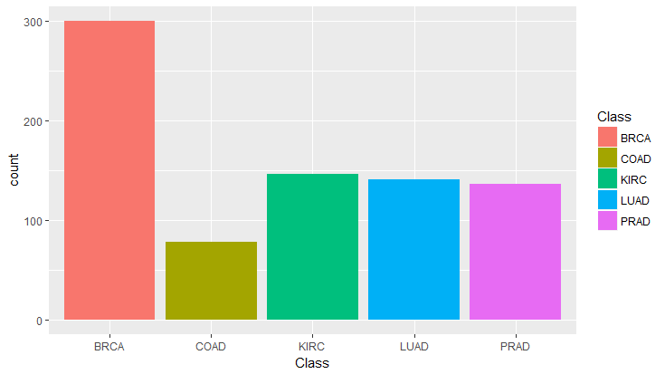
As shown in Fig.1, this data set is imbalanced with Colorectal cancer being the most underpresented. Taking this into account for multiclass classification, F1 score will be used to reflect the precision and recall performance within each class. There's also the issue of high dimensionality, where number of features (20,531 columns) far exceeds the number of samples (801 rows). A modified form of Principal Component Analysis (PCA) will be used to reduce the complexity of the dataset.
For a detailed explanation on Prinicipal Component Analysis (PCA), I highly recommend this link (it's the best I've seen and the visual is awesome!). Briefly, PCA is a technique commonly used to reduce high dimensional numerical data to lower dimensional space. Eigen decomposition of the feature covariance/correlation matrix results in the eigenvector matrix and its correpsonding eigenvalue matrix. Traditional PCA works by combining all original features with linear weights (aka: loadings) to capture the maximum variance of the data. Loading values can be obtained by eigenvector*square root (eigenvalue).The analysis results in several principal components, which are ranked by the amount of variance it captures (first PC captures the most). Each Principal Component(PC) will have its own eigenvector and eigenvalues that characterizes the variance, and each PC will have its own loadings for transforming the original data. For example, to calculate the first PC score for one sample, let Ci,j be the loadings for the i-th PC and the jth FPKM-normalized gene expression feature:
PC1 Score = gene_measurement{1} x C1,1 + gene_measurement{2} x C1,2 +... gene_measurement{j} x C1,j
When we are dealing with genomic data such as gene expression measurements, typically there's hundreds of thousands to
millions of gene or transcript being quantified per sample. Based on existing literature, we know that only a fraction of those
genomic features are driving the target of interest. To apply this constraint and
to select sub group of features, we can use sparse PCA which results in sparse loadings. Sparsity of the loadings is
effectively a form of feature selection, and it offers practical advantages such as easier interpretation and the need for
less variable measurements, which can be costly in RNA sequencing. One of the well
known sparse PCA methods was published by Zou, Hastie, and Tibshirani in 2005[2]. In this paper,
they approached PCA as a
regression problem optimized by lasso shrinkage of the coefficients resulting in some loadings of zero values. In this example, I used the
nsprcomp package in R, which allows you to specifiy the maximum number of non-zero loadings for each PC (and optional constraint for non-negative loadings).
I picked 1000 (5% of the total number of genes), but it's a parameter that can be further optimized. The codes for sparse
PCA are shown below (complete R script can be found at the github repo).
I tried both traditional PCA ( prcomp() ) and sparse PCA to generate the plots in Fig.2.
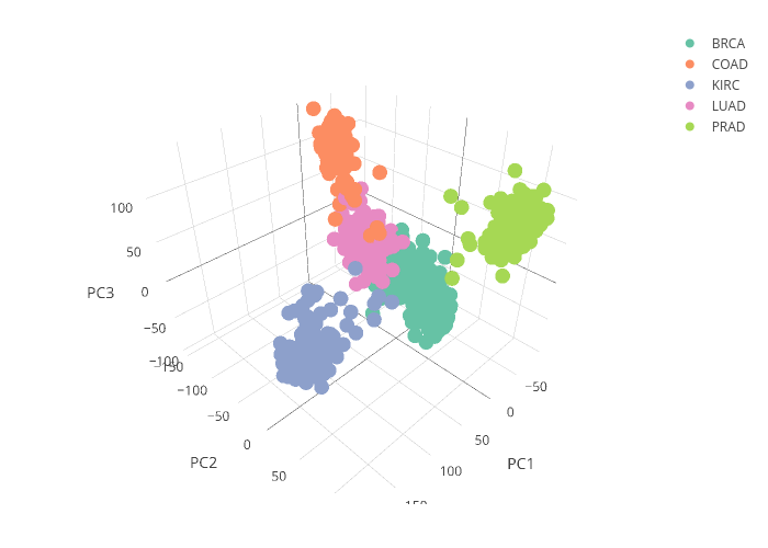
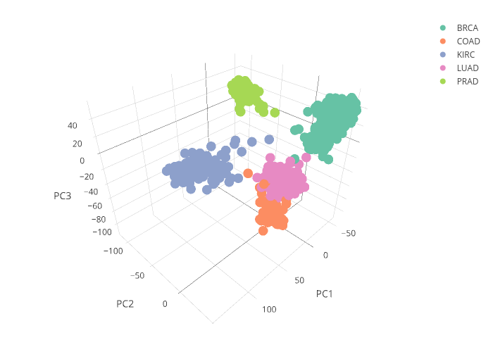
As shown above, the sparse PCA resulted in clear clustering of the groups along the PC axes, showing that selection of subgroup of gene expressions did not compromise the performance of the PCs.
XGB model of PC scores
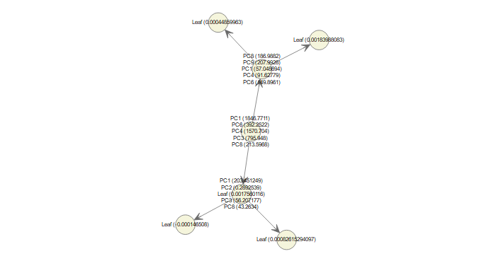
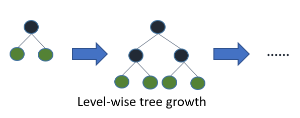
After getting the loadings for 1,000 gene expression features, 10 PC scores are computed for each sample. This would serve as the input matrix to the classification model Xtreme Gradient Boosting (XGB). In short, XGB is a regularized boosting algorithm in which the weak classifier learns its parameters based on the performance of the previous iteration, giving more weight to previously misclassified samples (or large error in case of regression) (see fig 3). The regularization in XGB helps to control for overfitting common in Gradient Boosting Machine (GBM) as boosting tries to reduce the bias of its learner.
Within each cross validation, sparse PCA is performed on training data only, and subsequent loadings are calculated for the validation data. At the end of each cross validations, the F1 scores of the predictions are obtained (Table 1). F1 score is the weighted average of precision and recall, and it's useful when you are working with an imbalanced dataset. The F1 value is calculated as 2*(precision*recall)/(precision+recall), and it reflects how precise and robust the classifier is.
| BRCA | COAD | KIRC | LUAD | PRAD | |
|---|---|---|---|---|---|
| CV 1 | 0.9833 | 0.9697 | 1.0000 | 0.9630 | 0.9824 |
| CV 2 | 1.0000 | 0.9677 | 0.9836 | 1.0000 | 1.0000 |
| CV 3 | 0.9600 | 0.9286 | 0.9824 | 0.9286 | 0.9615 |
| CV 4 | 0.9831 | 1.0000 | 1.0000 | 0.9655 | 1.0000 |
| CV 5 | 0.9836 | 0.9677 | 0.9830 | 0.9818 | 0.9811 |
Table 1. F1 scores of the 5 cross validation.
The classifications of Colorectal and Lung cancers have the lowest average (about 0.967) and wider variations (0.025). This is consistent with the plot of the PC scores shown in Fig.2, where the clusters of Colorectal cancer and Lung cancer are in close proximity, making it a bit harder to classify between these two cancers based on the gene expression data. Beyond this set of data related to tumor specimen gene expression, I think the approach described in this post can be extended to liquid biopsy of blood samples for prognosis of disease.
REFERENCES
[1].The Cancer Genome Atlas Research Network, Weinstein, J., Collisson, E.A., Mills,G.B., et al. The Cancer Genome Atlas Pan-Cancer analysis project, Nature Genetics 45, 1113–1120 (2013)
[2].Zou, H., Hastie, T., Tibshirani, R., Sparse Principal Component Analysis,Journal of Computational and Graphical Statistics, Volume 15, Number 2, Pages 265–286