The data set is from the Kaggle taxi ride data, and here's a snapshot:
| id | vendor_id | pickup_datetime | dropoff_datetime | passenger_count | pickup_longitude | pickup_latitude | dropoff_longitude | dropoff_latitude | store_and_fwd_flag | trip_duration (in seconds) |
|---|---|---|---|---|---|---|---|---|---|---|
| id2875421 | 2 | 2016-03-14 17:24:55 | 2016-03-14 17:32:30 | 1 | -73.98215 | 40.76794 | -73.96463 | 40.76560 | N | 455 |
| id2377394 | 1 | 2016-06-12 00:43:35 | 2016-06-12 00:54:38 | 1 | -73.98042 | 40.73856 | -73.99948 | 40.73115 | N | 663 |
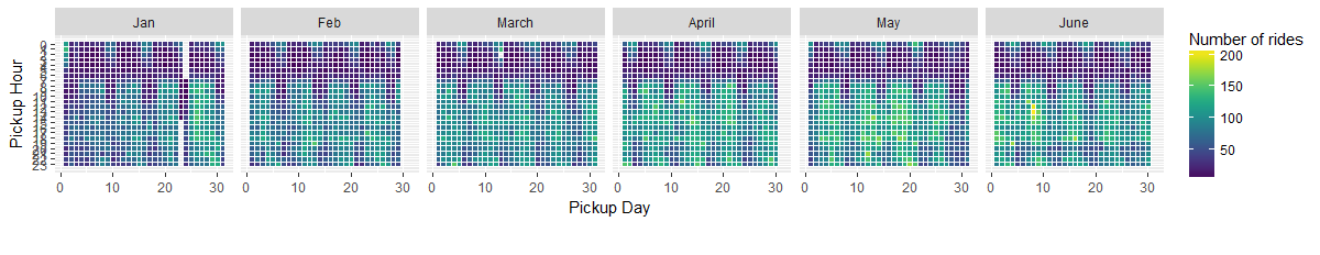
Often times, we need to extract time stamp elements from a data frame. In R, the lubridate package
is a fast and simple way to extract those information. This data set contains data on the scale ranging from
hour, weekday, date, and month. A good way to visualize that is using geom_tile() function within ggplot :
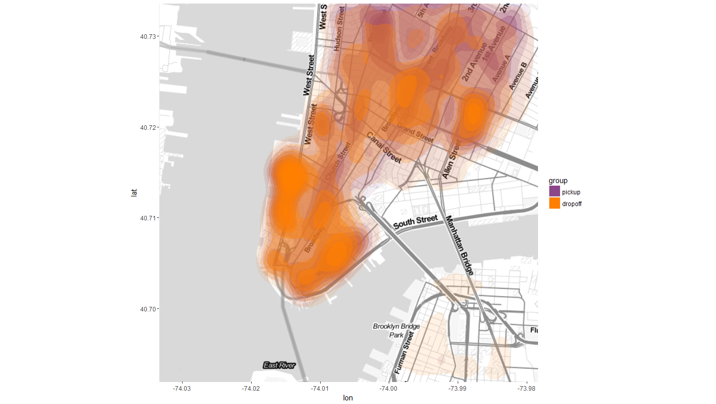
Now time for some contour plot, which requires both ggmap and ggplot libraries. ggmap
is used to retrieve the map of a locale using get_map()
Feature Engineering for Regression
Most of the time, machine learning workflows can benefit from feature engineering. Here, feature engineering is defined as adding or transforming relevant information/variables to the existing dataset in order to improve the model's learning and its performance. In some situations, feature engineering requires extensive domain knowledge, for this taxi dataset it was pretty straight forward. The new features obtained from the given features are the time stamp element (i.e, month, date, weekday, hour) and the haversine distance in km. The target variable, trip duration was log transformed since it displayed a highly skewered distribution. I generally prefer to have normal-ish distribution when working with continunous variable, because it helps some models to learn better. In fact, you might consider normalization/scaling to be a form of feature engineering because the raw data are transformed to optimize distance-based algorithms or gradient descend parameter updates.
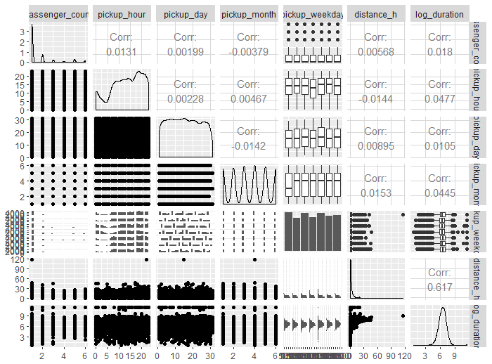
There's a useful library called GGally that offers a simple one-liner function for matrix scatter plots, along with display of distribution and correlation values. This is super useful for exploratory data analysis to get a sense of the data I'm working with. As shown in Fig 3 below, the strongest correlation was for one of the feature engineered variables - haversine distance.
library(GGally)
#using only 10K data points so it doesn't take too long to plot
sample_data<-datasets[1:10000,]
ggpairs(sample_data[, c("passenger_count","pickup_hour","pickup_day", "pickup_month", "pickup_weekday","distance_h", "log_duration")])
Caret and the Forest
After the data are preprocessed, I used the Caret library to perform grid search with cross validation (CV). I chose Random Forest (RF) regressor because it is known to work well with nonlinear data, it selects random subset of features at each node split, and it reduces variance (aka: overfitting) of the model by having independent weak learner trees.
Since the trees in RF are independent of each other, it is easy to setup parallel computing. This is helpful for running RF on large dataset with ~1M samples. On the Caret documentation, the author only mentioned doMC for parallel computing but that only works for Macs. I have a windows 10 laptop with 4 cores (8 processors), and found that the doParallel package worked well with the CV workflow.
Running the model fit on only 400K samples (to save time), the average validation RMSE was around 0.4135. There's still room for improvement, especially by running the whole training set. As you can see, it's easy to perform cross validated parameter tuning on a Random Forest regressor through Caret, which comes with other widely used models such as SVM, Logistic Regression, and GLM regression, etc (total of 238).