
Using R studio, the three methods I will compare are: K Nearest Neighbor (KNN), Random Forest (RF) imputation, and Predictive Mean Matching (PMM). The first two methods work for both categorical and numerical values, and PMM works best for continuous numerical variable. I chose to go with R for this task, because the last time I checked, Python does not have well-documented, hassle-free packages for these three methods. The closest thing I saw was fancyimpute0.3, but it did not offer RF and PMM.
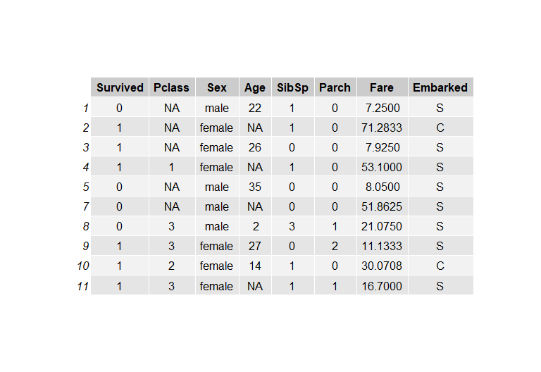
For the purpose of this post, I used the Titanic dataset, which contained a mix of categorical, ordinal, and numeric variables, and the Air Quality dataset (all numeric values). The Titanic dataset has 714 rows of samples, and the columns of interest are Survived, Pclass, Sex, Age, SibSp, Parch, Fare, and Embarked. I wanted to see the sensitivity, if there's any, of each imputation algorithm to percentage of missing values. For a given percentage, I randomly sample the row data for features PClass (Passenger Class) and Age, and set those values to NA (this would be considered Missing Not at Random). This was done for 10%, 20%, 30%, and 40% missing values for both columns, and Fig.1 shows a snapshot of the dataframe.
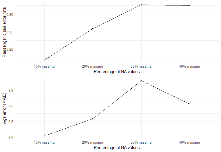
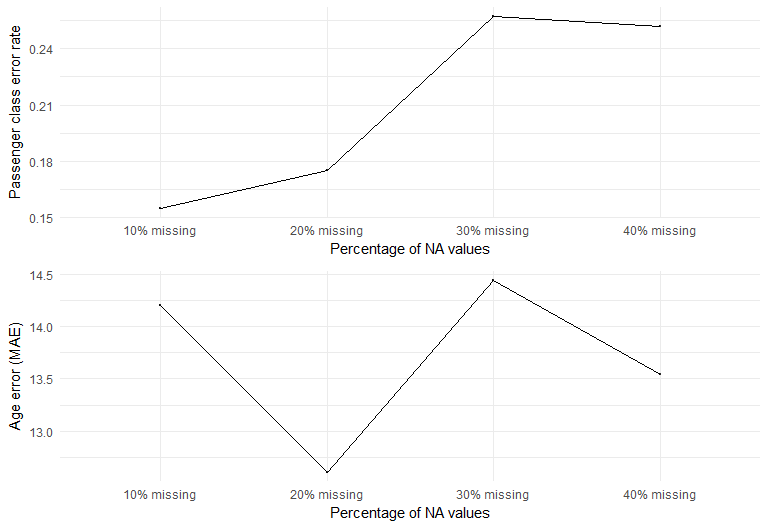
In evaluating performance, I used (1-accuracy) to represent the error for Pclass imputation, and Mean Absolute Error (MAE) for the Age imputation. I chose MAE after seeing that the distribution of the Age feature was normal-ish. For non-normal skewed distribution, it's recommended to use Root Mean Square Error (RMSE) instead.
K Nearest Neighbor (KNN)
Like its classifier counterpart, KNN is a non-parametric method that estimates missing value by finding the K nearest neighbors in feature space, then assign the class by majority vote of its K nearest neigbors. For regression, the value is the weighted average/median of its K nearest neighbors based on the distance.
But how do we measure the distance between samples in feature space? For numeric variables, it's common to use euclidean distance (l2 norm). However, imputing missing value often requires using information from categorical variables, so Gower's distance is designed to accomodate both numeric and categorical values in measuring dissimilarity. For the knn imputer in R library VIM, the Gower's distance between a pair of samples i and j is defined as : d_g(i,j) = sum_k(W_ijk * d_k(i,j) ) / sum_k(W_ijk).
Here, d_k(i,j) denotes distance between the value of variable k between the two samples. For categorical variable, d_k is 0 when the values between a pair of sample points are the same, otherwise it's 1. On the other hand, when working with numeric data d_k is calculated as 1-[(x_i-x_j)/(max(x)-min(x)] [1]. The weight W_ijk=1 when values of kth variable are present in both samples, otherwise it's 0. The Gower's matrix, d_g(i,j) is used to identifiy the k (default k=5) nearest neighbors for a give sample i.
Random Forest Imputation
Next, I tried imputation on the same data set using Random Forest (RF) algorithm. RF estimates missing value using growing a forest with a rough fill-in value for missing data, then iteratively updates the proximity matrix to obtain the final imputed value [2]. According to Breiman et al., the RF imputation steps are as follow:
- Replace missing values by average/mode in training data (initial step).
- Repeat in x iterations
- Train RF (including imputed values) on column j with the original missing data.
- Compute proximity matrix
- Update the missing value estimate with the proximity matrix as weights - for regression it's weighted average, and for categorical variables it's the weighted mode
- For test data, caculate proximities of test dat w/ respect to the training data.
The key of this algorithm lies in the proximity matrix. For n number of samples in the training set, it's a nxn matrix that shows how similar
one sample i is to another sample j. In each iteration, if sample X_i and X_j end up in the same terminal node of a tree within the
grown forest, then their proximity value P(i,j) is increased by 1. The matrix is often normalized by dividing by the number of trees, since that's a
tunable parameter. For my code ,the optimal number of trees was 40. In the MICE package, the function mice()
has the option for multiple imputation datasets (specified by the m variable).
Both of the non-parametric methods KNN and RF work using the "neighborhood" scheme. In general, these algorithms are based on this relationship:

Here, W(x_i,x') is the similarity/distance matrix relating a new test sample x' to x_i, then estimating y' based on y_i. For RF imputation, the proximity matrix is very sensitive to the complexity of the trees grown, and RF consists of so many hyperparameters (i.e., number of randomly sampled variables, subset sample size, and node size). According to a paper published by Lin and Jeon, the neighborhood mapped out by RF is largely determined by the local importance of each feature within a node[3]. This makes sense because RF imputation is optimized for nonlinear data.
Predictive Mean Matching (PMM)
The third method I want to explore is Predictive Mean Matching (PMM), which is commonly used for imputing continuous numerical data. The imputation works by randomly choosing an observed value from a donor pool whose predicted values are close to the predicted value of the missing case. The regression-based method works as follows to estimate missing values in variable Y:
- Use a set of variables X (with no missing data) to fit a linear regression on Y (choose cases of Y with no missing value) with coefficients B.
- To account for uncertainty of the coefficients, randomly sample for new set of regression coefficients B* by drawing from the normal distribution with mean of B and variance of B.
- Predict values for all cases of X using B*.
- For every missing case of X, find a group of K non-missing cases whose predicted values are close to the predicted value of the missing case. This is called the 'donor pool'.
- Randomly assign the observed value of a donor to replace the missing case.
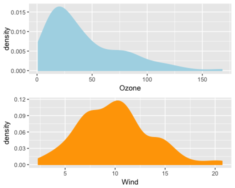
In theory, PMM works well on skewed data distribution because it's matching observed real value to the missing value. I tried PMM on the air quality public dataset, where both columns Ozone and Wind contain NA values, and the Ozone variable has a skewed distribution.
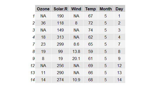
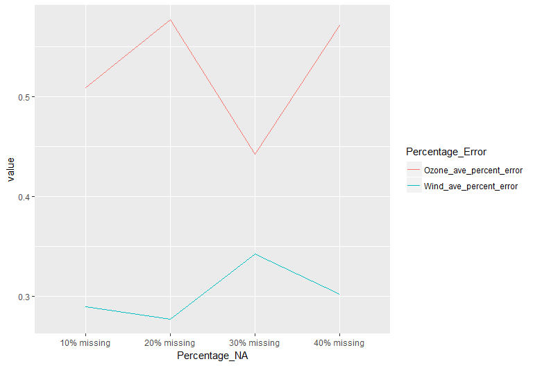
However, as shown in Fig.5. below, the percentage error of the Ozone imputation is higher and more volatile than that of the Wind features. And there appears to be a bit of a trade off between the imputation error of the two variables. While the matching of the value preserves the original distribution of the data, running linear regression on skewed data has some draw backs in producing reliable predicted values for downstream matching. Another issue is that the optimal k (number of donors) needs to be tuned because it varies depending on the dataset and number of samples (I used the default 5)[4]. The general rule of thumb is that with larger dataset, the imputation can benefit from a larger number of k.
Conclusion
After looking at the results from the three methods, it looks like the performances of KNN and RF are very sensitive to % of missing values. This is not surprising because these non-parametric algorithms impute based on finding its neighbors - and the more data observed the better the neighborhood can be mapped. Gower's matrix provided better imputation results for numerical data compared to RF, due to the way dissimilarity distance is calculated. However, RF performed better in categorical imputation. One way to approach the Titanic dataset is to use RF imputation on categorical variables and use KNN on numerical variables. However, it should be noted that RF imputation is computationally expensive. If computation cost is not a big concern, one way to account for uncertainty is to have multiple imputed datasets for model fitting, where the model outputs are averaged for prediction.
REFERENCES
[1]de Jonge,E., van der Loo, M., An introduction to data cleaning with R. 2013
[2]Breiman, L., Cutler, A. Random Forest. https://www.stat.berkeley.edu/~breiman/RandomForests/cc_home.htm
[3]Lin, Yi; Jeon, Yongho (2002). Random forests and adaptive nearest neighbors (Technical report). Technical Report No. 1055. University of Wisconsin.
[4]Allison,P., Imputation by predictive mean matching:promise & perils.Statistical Horizons Blog (https://statisticalhorizons.com/predictive-mean-matching)