The Art of Machine Learning

To better understand Bayesian statistics I recommend this great 'laymen' article published in New York Times. The gist can be captured by this quote "The essence of the frequentist technique is to apply probability to data. If you suspect your friend has a weighted coin, for example, and you observe that it came up heads nine times out of 10, a frequentist would calculate the probability of getting such a result with an unweighted coin [null hypothesis]. The answer (about 1 percent) is not a direct measure of the probability that the coin is weighted; it’s a measure of how improbable the nine-in-10 result is — a piece of information that can be useful in investigating your suspicion. By contrast, Bayesian calculations go straight for the probability of the hypothesis, factoring in not just the data from the coin-toss experiment but any other relevant information — including whether you have previously seen your friend use a weighted coin." In a mathematical sense, frequentist does repeated sampling to estimate an underlying parameter, and treats that parameter as fixed. In the Bayesian world, you can parameterize prior belief and the underlying distribution of observed data, and that belief can be updated with each new observation (posterior probability), and be described as a degree of belief. In this case, it's the data that is fixed (i.e., you're concerned with the probability of the outcome of one event).

Probabilistic Programming

Bayesian theory is the foundation for Probabilistic Programming, which 'learns' the parameters of interest using sophisticated sampling techniques (as oppose to solving linear equation using OLS), and returns a probability distribution of the parameters. To give a concrete example, suppose you have a linear equation y=w1*x+w0 and the goal is to find the weights (w0, w1). In order to estimate these parameters, you will need a sampling algorithm to search for the parameter value within a distribution that's updated throughout iterations. In the end, the weights(w0, w1) will be in the form of probability distributions, and predicted values will be derived from sampling of those distributions. One of the most common algorithms used is Markov-Chain-Monte-Carlo (MCMC) sampling. The general steps are outlined below [1]:

set up prior distributions for weights w0, w1.
sample from the probability distribution to get a vector of values for the weights (w).
Generate prediction values(y^), and calculate the loss term using the negative log of the likelihood distribution.
Update the weights distribution through minimization of the loss function.
Repeat the sampling process to get better estimation of the weights by proposing new values of vector w close to the previous values. The MCMC method moves along the joint distribution according to some pre-defined threshold values (e.g., current loss/previous loss ratio <1).

The MCMC method is very computationally expensive. To make it more efficient, an improvement was made in the form of Hamiltonian Monte Carlo method(HMC), which takes advantage of the gradient of the log posterior-density to guide the sampling toward region of higher likelihood. No-U-Turn Sampler (NUTS) was a more recent improvement on top of HMC, it offers adaptive tuning of hyperparameter values for determining number of steps and step size[2].

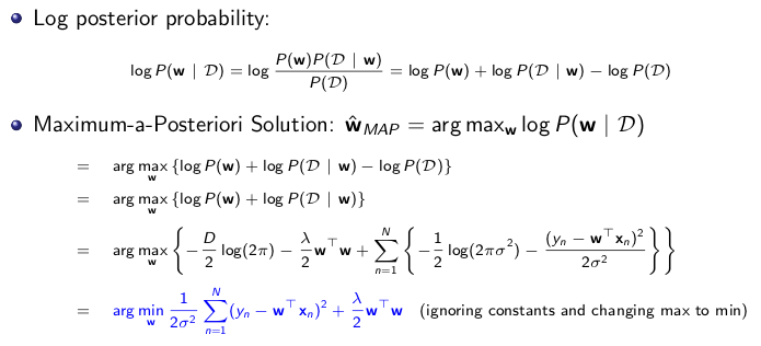
To better understand how loss term is related to the log likelihood, I found a ppt lecture given by Dr. Piyush Rai for CS5350/6350 at the University of Utah. As shown in Fig.1., the takeaway is that log of posterior distribution (P(w|D)) is maximized by looking for the optimal w, and argmax(log P(w|D) is equivalent to argmin of (-log P(D|w)-log(P(w)). This set up showes that negative log of the likelihood function is the loss term, and negative log of w serves as regularization term. With auto differentiation, the gradient of the -log P(D|w) can be found to faciliate more efficient sampling for w.

PyMC3

As stated in the PyMC3 tutorial, NUTS is best used for continuous parameter sampling, and Metropolis for categroical parameter. In the figure below, I share an example of running a logistic model consists of both continuous and categorical inputs to produce a binary outcome value. I find that the easiest way to incorporate mixed data type in PyMC3 is to define your own function (instead of using the default pm.glm.GLM() function).

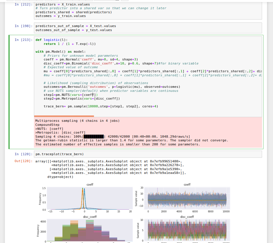
In defining the distribution of the categorical variables (there were 7), either Bernoulli or Binomial distributions can be used. With pm.Binomial(), user must enter number of trials (e.g., n=10) since Binomial function is concerned with number of trials. Another useful feature of PyMC3 is that user can define multiple steps to assign different sampling method to the desired variable(s). It's also helpful to use the share() function from PyMC3 to later share the out-of-sample test data in order to run inference on the trained model(see code below).


############### after model is trained #############

#switch variable values to predictors_out_of_sample data, then run model by sampling 200 times for each data point
predictors_shared.set_value(predictors_out_of_sample)
ppc = pm.sample_ppc(trace_bern, model=model, samples=200)

# To generate a final prediction value, use beta function to characterize the prediction distribution.
# beta distribution is frequently used in Bayesian statistics, empirical Bayes methods and classical statistics to
#capture overdispersion in binomial type distributed data. when n(number of samples in code above) =1, then
#it's bernoulli distribution
β = st.beta((ppc['outcomes'] == 1).sum(axis=0), (ppc['outcomes'] == 0).sum(axis=0))
pred_eval=pd.DataFrame({'ppc_pred':β.mean(), 'actual_value':y_test.values})

Conclusion

With sufficient samplings, Bayesian modeling outperformed regular logistic regression fitting by a slight margin in F1 score. Given the computational cost, it would be more efficient to apply probabilistic programming to complex model with higher dimensions than the dataset used for the code presented here. Currently there's great interest in training models with Bayesian Neural Network that is capable of generating prediction/posterior distributions, and yielding higher accuracy[3]. However, within PyMC3 there's been some issues with saving the model and the trace file - when user reloads it to run on new dataset it doesn't accept the new data (i.e., failing due to broadcasting different sample length). Hopefully PyMC3 and other packages like Edward would roll out improvements for more robust backend support.

REFERENCES

[1]Sedar, J., Bayesian Inference with PyMC3 - Part 1. https://blog.applied.ai/bayesian-inference-with-pymc3-part-1/

[2]Hoffman, M.D., Gelman, A. (2011). The No-U-Turn Sampler: Adaptively Setting Path Lengths in Hamiltonian Monte Carlo .

[3]Mullachery, V., Khera,A., Husain, A. (2018). Bayesian Neural Networks.